Redrawing the Boundary between Organism and Environment
This page provides supplementary materials to accompany the paper "Redrawing the Boundary between Organism and Environment", to appear in the Proceedings of the Ninth International Conference on the Simulation and Synthesis of Living Systems (ALIFE IX), edited by J. Pollack et al., MIT Press, 2004 (forthcoming).
EvoCA-A
[Experimental Details] [Example Results] [Source Code]Experimental Details
General Design
(Further details about the design of EvoCA-A can be found in the paper The Control of Dynamical Systems by Evolved Constraints).
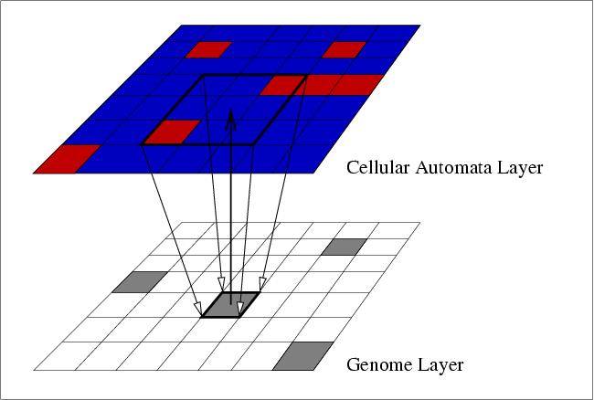
A standard generational genetic algorithm is used to evolve a population of individuals. Each individual is evaluated in isolation, and placed in the same grid position in Layer 2 (the genome layer). The iteration count of the CA is reset to zero at the start of each evaluation. The CA layer (Layer 1) ran the standard "Game of Life" dynamics with two states (state 0, the quiescent state, and state 1, the "live" state). All cells are initially set to the quiescent state, except those which have non-quiescent states specified by timed genes acting at time zero, or those that are influenced by external signals (described later). The CA is then allowed to run for a given number of iterations, with the genes of the genome setting specific cell states when they become active. The fitness function is described later.
To generate the initial population of P individuals, a set of Pi individuals (where Pi >= P) is randomly generated and evaluated. The fittest P individuals from this set are selected to fill the initial population.
The genetic algorithm can be set up to use either tournament selection or fitness proportional (roulette wheel) selection. Elitism may also be applied, in which case the fittest individual from the population is guaranteed to pass at least one exact copy of itself into the next generation.
In addition to one-point crossover and gene mutation, a number of other genetic operators
are also available: gene insertion (a random gene is inserted into an existing genome); gene
deletion (an existing gene is deleted from a genome); gene reversal (the order of a sequence
of genes between two selected points in the genome is reversed); and gene duplication (a
sequence of genes between two selected points in the genome is duplicated at the end of the
genome). A limit on the maximum allowable genome length is defined. This is respected
both during the initial generation of random genomes and in the action of the genetic
operators.
Sensor and Effector Evolution Experiments
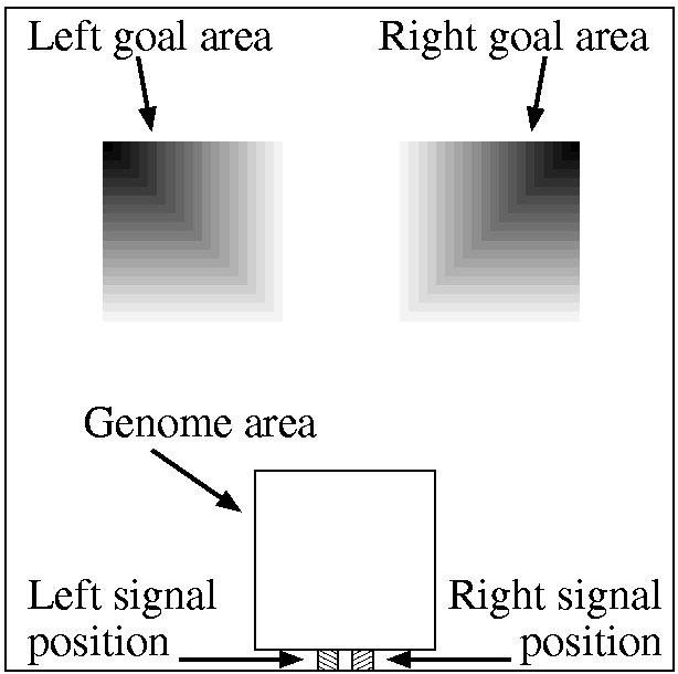
The following example demonstrates the application of the approach to the topic of sensor and effector evolution. The system was set up as shown in the picture below, using a 2D toroidal CA of size 75x75 cells. To evaluate a genome, it was placed in the centre of the genome area shown. The maximum radius of gene action is shown by the boundary of this area (i.e. genes could directly set the state of only those cells within the genome area). In addition, two goal areas were defined, along with two signal positions, as shown. Note that the signal positions adjoin, but do not overlap, the genome area. The task that the organisms were set is described below. Each genome was tested under three conditions: left signal, right signal, and no signal.
For the left signal condition, the cells in the 2x2 left signal position (see picture) were initially set to state 1 (the non-quiescent state). In this condition, the task of the organism was to produce activity in the left goal area. Any activity in this goal area over the course of the evaluation was rewarded, with the darker shaded cells (see picture) being rewarded more than the lighter cells in the goal area. However, any activity in the right goal area was penalised.
At each iteration, the fitness of the organism was incremented for each cell in goal area which was in the non-quiescent state. Furthermore, activity in some cells in the goal area was rewarded more than in others -- in the picture, the darker the cell in the goal area, the higher the reward. However, non-quiescent activity in the right goal area was scored in the same way, and the total increment (or decrement) in fitness at each iteration was the score gained in the left goal minus that gained in the right goal. The organism was evaluated for a fixed number of iterations, and its final fitness score, FL, was its cumulative score from each iteration. Thus, in the left signal condition, organisms were rewarded for causing activity in the left goal area, and punished for causing activity in the right goal area.
For the right signal condition, the opposite signal positions and
goal areas were used in the fitness calculation.
For the no signal condition, any activity in either goal area was
penalised. The final fitness FN
was calculated as zero minus the cumulative scores for activity in both of the goal
areas, i.e. organisms were punished for causing activity in either goal area.
The combined fitness for all three conditions was calculated as F = max( (FL + FR)/2 + FN , 0).
The main parameter values used in these trials were as follows:
Population Size P=500, Generations 150, Iterations per Evaluation
200.
Full details of all parameter settings are given in the following parameter files:
| Run |
Parameter File |
RNG Seed |
Evolved Genome |
|---|---|---|---|
| Glider |
evoca_glider_params.txt |
1050318375l |
evoca_glider_winner.dat |
| Spreading Activation |
evoca_sprdact_params.txt |
1050680650l |
evoca_sprdact_winner.dat |
Example Results
| Evolved
Glider Click on the link above to see a movie of an organism that achieves the task by producing a "glider" that travels in the appropriate direction. The movie is divided into three sections: in the first, a signal is initially present in the left signal position; in the second, a signal is initially present in the right signal position; in the final section of the movie, no signal is provided. The organism responds appropriately in each case. Remember that the environment wraps around at the borders, so activity that "falls off" the bottom of the grid reappears at the top. Note that some movie players seem to have a problem with this movie (sometimes it gets cut off before it has finished). You could try downloading it and running it from your local computer, or try using a different mpeg player. This movie is now available on YouTube! |
 |
Evolved
Spreading Activation Click on the link above to see a movie of another organism evolved for the same task as the glider organism. In this case, the organism causes a much more extensive pattern of activation in the appropriate goal area, and therefore achieves much higher fitness than the glider organism. Note that some movie players seem to have a problem with this movie (sometimes it gets cut off before it has finished). You could try downloading it and running it from your local computer, or try using a different mpeg player. This movie is now available on YouTube! |
| Experimental Task Setup |
Source Code
- evoca_gol_v1.tgz (gzipped tar file containing source code, 39KB)
- README file (also included in the tar file above)
EvoCA-B
[Experimental Details] [Example Results] [Source Code]
Experimental Details
In these experiments, the CA Layer was again running the standard 2-state "Game of Life"
rules. In contrast to the EvoCA-A experiments, multiple genomes coexisted in the Genome
Layer, as described in the paper. A 100x100 CA grid was used, and the run was initiated
with 100 randomly generated genomes placed at random positions. The source code, which
includes details of all parameter settings, is provided below.Example Results
The following movie shows an example of EvoCA-B in action. What you see is a CA running Game of Life dynamics. What you don't see is that there is also a population of genomes (initially 100 of them, each randomly generated and placed on a random cell in the CA), each influencing the dynamics by setting the cell's state when their genes are activated. Some local environments (i.e. local configurations of the CA) promote a genome's stability and chances of reproduction, and others inhibit them. There is therefore a loop from genomes influencing the dynamics of the environment, and back from the environment supplying selection pressure for particular genomes. At first, the dynamics appear to be chaotic. However, about half way through the movie you see something interesting start to happen; the emergence of genomes which generate local environments which promote their own survival. This is evidenced by regions of more stable dynamics in the system; these are genome-regulated self-stabilising dynamics (a significant step towards the origin of life). These genomes, and their associated dynamics (phenotypes) eventually spread throughout the whole system by natural selection.
- Download EvoCA Movie [MPEG] (Size 14.6MB)
-
- N.B. Some versions of Microsoft Media Player do not seem to be able to play this movie. Also, on some players it gets cut off before the whole thing has played. If you experience problems, you could try using QuickTime player, another version of Media Player, or a Unix/Linux player such as mpeg_play. It also may help to download the file first and then play it from your own computer.
- This movie is now available on YouTube!
Source Code
- evocab_v0p11.tgz (gzipped tar file containing source code, 10KB)
- README file (also included in the tar file above)
Tim Taylor, 27 April 2004 (page last updated: 14 January 2010)